Identifying Critical Neurons in ANN Architectures using Mixed Integer Programming
Publications ·In this research, we attempt to understand the neural model architecture by computing an importance score to neurons. The computed importance score can be used to prune the model or to understand which features are more meaningful to the trained ANN (artificial neural network). The importance score is computed using Mixed Integer Programming (proposed method infographic) (Garey & Johnson, 1979).
What’s Mixed Integer Programming (MIP) ?
Mixed Integer Programming is a combinatorial optimization problem restricted to discrete decision variables, linear constraints and linear objective function. The MIP problems are NP-complete, even when variables are restricted to only binary values. The difficulty comes from ensuring integer solutions, and thus, the impossibility of using gradient methods. When continuous variables are included, they are designated by mixed integer programs.
The solver tries to search the space of possible solutions based on the set of input constraints. In order to narrow down the set of possible solutions, the solver uses an objective function to select the optimal solution. For a tutorial about mixed integer programs using python check introduction to mixed integer programming.
Proposed Framework diagram

- First we start by training the neural model to be pruned on the dataset.
- After training, we feed a batch of images (an image per class) to the MIP, and we compute a lower and upper bound at each layer for each input image. \(l = x - \epsilon\) and \(u = x + \epsilon\)
- We create a set of liner constraints representing the neural model with integer variable \(v\) used for ReLU activation constraint.
- We define the objective used by the MIP to sparsify more neurons with marginal loss in predictive accuracy.
- After running the solver and computing the neuron importance score, any neuron below a tuned threshold (0.1) is pruned and set to zero without fine-tuning.
In the following sections, we will explain in depth the constraints used, the objective and the generalization technique (to use masks computed by a dataset on another dataset).
MIP Constraints
Bounds propagation
We will propagate input images through each layer in the ANN, each image having 2 perturbed values \(x-\epsilon\) and \(x+\epsilon\) denoting initial upper and lower bound.
In our work, we use tight \(\epsilon\) value to approximate the input trained model and to narrow the search space used by the solver.
ReLU Constraints
We define the following decision variables :
- \(z_{i}\) -> decision variable defining value of input logit to layer \(i\)
- \(v_{i}\) -> binary decision variable as a gate for ReLU activation function (this variable can be relaxed to a continuous value for faster execution)
- \(s_{i,j}\) -> decision variable holding the neuron importance score at layer \(i\) with neuron index \(j\)
The following parameters are used :
- \(W_i\) -> fixed weights of layer \(i\)
- \(b_i\) -> bias of layer \(i\)
- \(u_i\) -> upper bound of output logit of layer \(i\)
- \(l_i\) -> lower bound of output logit of layer \(i\)
Now we define the constraints used :
\(z_0 = x\) Equality between input batch to the MIP and the decision variable holding input to the first layer. \(z_{i+1} \geq 0\) For ReLU activated layers, the output logit is always positive.
\(v_{i} \in \{0, 1\}\) Defining gating decision variable used for ReLU
\(z_{i+1} \leq v_i u_i\) Upper bound of current layer’s logit output using gating variable.
\(z_{i+1} + (1- v_i) l_i \leq W_i z_i + b_i - (1- s_i)u_i\) \(z_{i+1} \geq W_i z_{i} + b_i - (1- s_i)u_i\)
The above constraints contain the decision gating variable \(v_i\) that is choosing whether to enable the logit output or not along with the neuron importance score \(s_i\).
\(0 \leq s_{i} \leq 1\) The neuron importance score is defined in the range of [0-1]. Same constraints are used for convolutional layers with a computed importance score per feature map. We convert the convolutional feature map to a Toeplitz matrix, and the input image to a vector. Hence, allowing us to use simple matrix multiplication that can be efficiently computed, but with high memory cost.
Convolutional layer as Fully Connected
Toeplitz Matrix is a matrix in which each value is along the main diagonal and sub diagonals are constant. So given a sequence \(a_n\), we can create a Toeplitz matrix by putting the sequence in the first column of the matrix and then shifting it by one entry in the following columns. The following figure shows the steps of creating a doubly blocked Toeplitz matrix from an input filter (Brosch & Tam, 2015).
\[\begin{pmatrix} a_0 & a_{-1} & a_{-2} & \cdots & \cdots & \cdots & \cdots & a_{-(N-1)} \\ a_1 & a_0 & a_{-1} & a_{-2} & & & & \vdots \\ a_2 & a_1 & a_0 & a_{-1} & \ddots & & & \vdots \\ \vdots & a_2 & \ddots & \ddots & \ddots & \ddots & & \vdots \\ \vdots & & \ddots & \ddots & \ddots & \ddots & a_{-2} & \vdots \\ \vdots & & & \ddots & a_1 & a_0 & a_{-1} & a_{-2} \\ \vdots & & & & a_2 & a_1 & a_0 & a_{-1} \\ a_{(N-1)} & \cdots & \cdots & \cdots & \cdots & a_2 & a_1 & a_0 \\ \end{pmatrix}.\]
Feature maps or kernels at each input channel are flipped, and then converted to a matrix. The computed matrix when multiplied by the vectorized input image will provide the fully convolutional output. For padded convolution, we use only parts of the output of the full convolution, and for the strided convolutions we use sum of 1 strided convolutions as proposed by Brosch, Tom and Tam, Roger. First, we pad zeros to the top and right of the input feature map to have same size as the output of the full convolution. Then, we create a Toeplitz matrix for each row of the zero padded feature map. Finally, we arrange these small Toeplitz matrices in a large doubly blocked Toeplitz matrix. Each small Toeplitz matrix is arranged in the doubly Toeplitz matrix in the same way a Toeplitz matrix is created from the input sequence, with each small matrix as an element of the sequence.
The formulation will become \(\sum_{d=1}^{N^l}W^{(l)}_{d} h^{l-1}+b^{(l)}\) at each feature map. We then, incorporate the same constraints used for the fully connected layer repeated for each feature map.
Pooling Layers
Average Pooling
Pooling layers are used to reduce the spatial representation of an input image by applying an arithmetic operation on each feature map of the previous layer. We model both average and max pooling on multi-input units as constraints of a MIP formulation with kernel dimensions \(ph\) and \(pw\).
Avg Pooling layer applies the average operation on each feature map of the previous layer. This operation is just linear and it can be easily incorporated into our MIP formulation: \(\begin{alignat}{3} x & = \text{AvgPool}(y_1,\ldots,y_{ph * pw} ) & = \frac{1}{ph * pw} \sum_{i=1}^{ph * pw} y_i . \end{alignat}\)
Max Pooling takes the maximum of each feature map of the previous layer. \(\begin{alignat}{3} x & = \text{MaxPool}(y_1,\ldots,y_{ph * pw} ) & = \text{max}\{y_1,\ldots,y_{ph * pw}\}. \end{alignat}\) This operation can be expressed by introducing a set of binary variables \(m_1, \ldots ,m_{ph * pw}\).
\[\begin{align} \sum_{i=1}^{ph * pw} m_i = 1 \\ x \ge y_i, \\ x \le y_i m_i+U_i(1-m_i) \\ m_i \in \{0,1\} \\ i=1, \ldots, ph * pw. \end{align}\](Fischetti & Jo, 2018) devised the max and avg pooling representation using a MIP. The max pooling representation contains a set of gating binary variables enabled only for the maximum value \(y_i\) in the set \(\{y_1, \ldots, y_{ph * pw}\}\).
MIP Objective
Sparsification
Our first objective is to maximize number of neurons sparsified from the trained model. The more neurons having zero importance score the better for this objective.
Let’s define a set of notation to make the equations easier :
- \(L_i\) set of neurons at layer \(i\).
- \(I_i\) be the sum of neuron scores \(s_{i,j}\) at layer \(i\) having \(\vert L_i \vert\) neurons scaled down to range \([-2, -1]\).
\(I_i = \sum_{j \in L_i} (s_{i,j} -2)\)
- Let \(A = \{I_{i} : i=1,\ldots,n\}\)
In order to create a relation between neuron scores in different layers, our objective becomes the maximization of the amount of neurons sparsified from layers having higher score \(I_i\).
\[\text{sparsity} = \frac{argmax_{A^{'} \in A, |A^{'}| = (n-1)} \sum_{I \in A^{'}} I}{\sum_i^{n} \vert L_i \vert}\]Marginal Softmax
Our second objective is to select which neurons are non-critical to the current model’s predictive task. For that objective, we use a simple marginal softmax computed on the true labels of the input batch of images.
In marginal softmax(Gimpel & Smith, 2010), the loss focus more on the predicted labels values without relying on the value of the logit.
The solver’s logit value will be weighted by the importance score of each neuron and will be different from the true one.
\(\text{softmax} = \sum_{j \in L_n} \log[\sum_c \exp(z_{j, n, c})] - \sum_{j \in L_n} \sum_c Y_{j,c} z_{j,n,c}\) Where index \(c\) stands for the class label.
Multi-Objective (MIP)
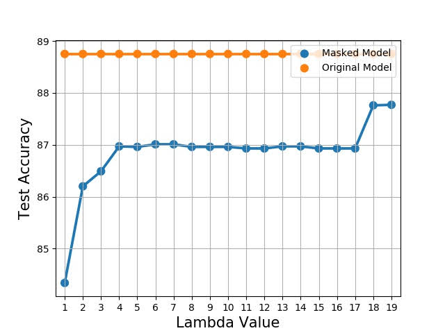
We define \(\lambda\) used to give more weight to the predictive capacity of the model. The \(\lambda\) is multiplied by the marginal softmax.
\[\text{loss} = \text{sparsity} + \lambda \cdot \text{softmax}\]The larger the value of the lambda the less pruned parameters.
Experiments
Generalization

In this experiment, we show that the computed neuron importance score on dataset \(d1\) with specific initialization can be applied on another unrelated dataset \(d2\) achieving good results.
Steps :
- We train the model on dataset \(d1\).
- We compute its neuron importance score using MIP
- After computing the neuron importance score, we create a masked neural model with neurons below certain threshold removed.
- We restart the model to its initialization while using its masked version.
- We train the masked version on \(d2\).
Pruning
We sparsify the model and compute its predictive accuracy on the equivalent dataset’s test set. Steps:
- We start by removing non-critical neurons having a score below certain threshold (0.1 in fully connected models and 0.2 in convolutional models) and then we evaluate the masked model (Ours).
- We remove random neurons from the model and evaluate for comparison purposes with our method (RP).
- We remove top scoring neurons denoted by the MIP from the model (CP).
- Another experiment, we try to fine tune our technique for 1 epoch to recover the lost predictive accuracy and in some cases it surpasses the original non-masked model (Ours + fine-tuning).
All the above pruning ways are having the same number of removed parameters as removing non-critical neurons.
Results
| Dataset | MNIST | Fashion-MNIST | CIFAR-10 | |
|---|---|---|---|---|
| Architecture | LeNet-5 | VGG-16 | ||
| Ref. | \(98.9\% \pm 0.1\) | \(89.7\% \pm 0.2\) | \(72.2\% \pm 0.2\) | \(\; \; 83.9\% \pm 0.4\) |
| RP. | \(56.9\% \pm 36.2\) | \(33\% \pm 24.3\) | \(50.1 \% \pm 5.6\) | \(\; \; 85\% \pm 0.4\) |
| CP. | \(38.6\% \pm 40.8\) | \(28.6\% \pm 26.3\) | \(27.5\% \pm 1.7\) | \(\; \; 83.3\% \pm 0.3\) |
| Ours | \(\mathbf{98.7\% \pm 0.1}\) | \(\mathbf{87.7\% \pm 2.2}\) | \(\mathbf{67.7\% \pm 2.2}\) | N/A |
| Ours + ft | \(\mathbf{98.9\% \pm 0.04}\) | \(\mathbf{89.8\% \pm 0.4}\) | \(\mathbf{68.6\% \pm 1.4}\) | \(\; \; \mathbf{85.3\% \pm 0.2}\) |
| Prune (\%) | \(17.2\% \pm 2.4\) | \(17.8\% \pm 2.1\) | \(9.9\% \pm 1.4\) | \(\; \; 36\% \pm 1.1\) |
| threshold | \(0.2\) | \(0.2\) | \(0.3\) | \(0.3\) |
The solving time is in terms of second, but if we relax \(v_i\) to be continous instead of binary the solver will take less than a second (relaxation of the constraints).
Generalization Results
| Model | Source | Target | Ref. Acc. | Masked Acc. | Pruning |
|---|---|---|---|---|---|
| LeNet-5 | Mnist | Fashion MNIST | \(\; \;89.7\% \pm 0.3\) | \(\; \;89.2\% \pm 0.5\) | \(\; \;16.2\% \pm 0.2\) |
| CIFAR-10 | \(\; \;72.2\% \pm 0.2\) | \(\; \;68.1\% \pm 2.5\) | |||
| VGG-16 | CIFAR-10 | MNIST | \(\; \;99.1\%\pm0.1\) | \(\; \;99.4\%\pm0.1\) | \(\; \;36\% \pm 1.1\) |
| Fashion-Mnist | \(\; \;92.3\% \pm 0.4\) | \(\; \;92.1\% \pm 0.6\) |
The masked version of the model was computed on MNIST dataset, these results shows that computed sub-network on a dataset can be applied and generalized to another dataset (with no statistical relation between both datasets).
Discussion
We have discussed the constraints used in the MIP formulation and verified the score produced by the MIP by a set of experiments on different types of architectures and datasets. Furthermore, our approach was able to generalize on different datasets.
Check the paper for more theoretical details (ElAraby et al., 2020).
Collaborators
References
- ElAraby, M., Wolf, G., & Carvalho, M. (2020). Identifying efficient sub-networks using mixed integer programming. OPT Workshop, 3.
- Fischetti, M., & Jo, J. (2018). Deep neural networks and mixed integer linear optimization. Constraints An Int. J., 23(3), 296–309. https://doi.org/10.1007/S10601-018-9285-6
- Brosch, T., & Tam, R. C. (2015). Efficient Training of Convolutional Deep Belief Networks in the Frequency Domain for Application to High-Resolution 2D and 3D Images. Neural Comput., 27(1), 211–227. https://doi.org/10.1162/NECO_A_00682
- Gimpel, K., & Smith, N. A. (2010). Softmax-Margin CRFs: Training Log-Linear Models with Cost Functions. Human Language Technologies: Conference of the North American Chapter of the Association of Computational Linguistics, Proceedings, June 2-4, 2010, Los Angeles, California, USA, 733–736. https://aclanthology.org/N10-1112/
- Garey, M. R., & Johnson, D. S. (1979). Computers and Intractability: A Guide to the Theory of NP-Completeness. W. H. Freeman.