Predicting The Generalization Gap In Deep Networks With Margin Distributions
Paper Review ·In this paper (Jiang et al., 2018), they discuss a method that can predict the generalization gap from trained deep neural networks. The authors used marginal distribution information from input training set as a feature vector used by an estimator to get the generalization gap.
The authors used marginal bounds extracted from each data point in the training set to represent a marginal distribution. The extracted marginal distribution used as input feature to train an estimator on the generalization gap. Next we explain the generalization and the marginal distribution used in predicting it.
What’s the generalization gap?
The generalization gap can be defined as the difference in terms of DNN’s performance between training set and testing set. This difference comes from the distributional shift between collected training data and real test data.
What’s marginal distribution?
We start by explaining the concept of the marginal bound.
Marginal Bound
The marginal bound is the distance between the data point and the decision boundary (Elsayed et al., 2018). In other words, the marginal bound is the smallest displacement of the data point that results in a score tie between the top two classes i and j. In this work, they only consider positive marginal bounds (only correctly predicted training data points.) \(D_{(f, x, i, j)} \triangleq \{x | f_i(x) = f_j(x)\}\) \(D_{(f, x, i, j)} \triangleq min_{\delta} ||\delta||_p s.t. f_i(x + \delta) = f_j(x + \delta)\)
Decision boundary
In SVM we can compute the distance of the data point to the decision boundary. However, in DNNs, it is intractable to compute the exact distance to the decision boundary. a first order Taylor approximation is used to approximate the distance to the decision boundary. Then, the distance of the data point to the decision boundary at layer (l) is denoted by: \(D_{(f, x, i, j)}(x^l) = \frac{f_i(x^l) - f_j(x^l)}{||\nabla_{x^l}f_i(x^l) - \nabla_{x^l} f_j(x^l)||_2}\)
Here \(f_i(x^l)\) represents the output logit at class \(i\) for input representation \(x^l\) at layer \(l\). The distance can be simply negative, if its corresponding data point is on the correct or wrong side of the decision boundary.
If we use statistics properties on the marginal bound to represent the trained DNN, our computed distance will depend on the scaling factor at each layer (in case it is multiplied or divided by a constant). Hence, we need to normalize the marginal bound of each network before feeding it to the estimator \(\hat{f}\).
Normalizing Marginal bound
In order to normalize the marginal bounds, let \(x_k^l\) be the representation vector of data point \(x_k\) at layer \(l\). We then compute the variance of each coordinate of \(\{x_k^l\}\), and then sum these individual variances. More concretely, the total variation is computed as:
\[\begin{equation} \nu (\boldsymbol{x}^{l}) = \text{tr} \Big(\frac{1}{n} \sum_{k=1}^n (\boldsymbol{x}_k^l - \bar{\boldsymbol{x}}^l) (\boldsymbol{x}_k^l - \bar{\boldsymbol{x}}^l)^T \Big) \quad , \quad \bar{\boldsymbol{x}}^l = \frac{1}{n} \sum_{k=1}^n \boldsymbol{x}_k^l \,, \end{equation}\]Using the total variation, the normalized margin is specified by: \(\begin{equation} \hat{d}_{f, (i,j)}(\boldsymbol{x}_k^l) = \frac{d_{f, (i,j)}(\boldsymbol{x}_k^l)}{\sqrt{\nu (\boldsymbol{x}^{l})}} \label{eq:tv_norm_margin} \end{equation}\)
Marginal Distribution Signature
Finally, to create a signature for the marginal distribution, the authors extract statistical properties from the margin bound of correctly predicted training data points. Given a set of distances \(\mathcal{D} = \{\hat{d}_m\}_{m=1}^n\), which constitute the margin distribution. They use the median \(Q_2\), first quartile \(Q_1\) and third quartile \(Q_3\) of the normalized margin distribution, along with the two {fences} that indicate variability outside the upper and lower quartiles. There are many variations for fences, but in this work, they used \(IQR = Q_3 - Q_1\), with upper fence to be \(\max(\{\hat{d}_m : \hat{d}_m \in \mathcal{D} \wedge \hat{d}_m \leq Q_3 + 1.5IQR\})\) and the lower fence to be \(\min(\{\hat{d}_m : \hat{d}_m \in \mathcal{D} \wedge \hat{d}_m \geq Q_1 - 1.5IQR\})\).
Linear estimator
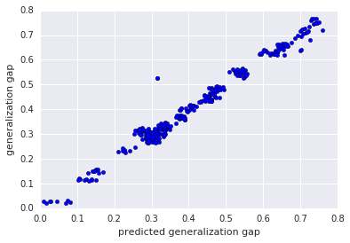
These 5 statistics extracted at first four layers and fed to the linear regression estimator \(\hat{f}\) result in a decent generalization gap predictor.
Dataset
The dataset used in that work is provided at Demogen, and my re-implementation at Generalization gap features
Conclusion
Here, the authors managed to get a feature that represents the separability of representations, this feature was used as a feature vector to predict the generalization gap based only on a subset of the training set.
Side Note
I would recommend reading the paper itself and checking the related work, this is just a summary to give you a rough idea of what is going on.
References
- Jiang, Y., Krishnan, D., Mobahi, H., & Bengio, S. (2018). Predicting the Generalization Gap in Deep Networks with Margin Distributions. CoRR, abs/1810.00113. http://arxiv.org/abs/1810.00113
- Elsayed, G. F., Krishnan, D., Mobahi, H., Regan, K., & Bengio, S. (2018). Large Margin Deep Networks for Classification. CoRR, abs/1803.05598. http://arxiv.org/abs/1803.05598